Getting Started
To use hasasia, first import these useful modules:
import numpy as np
import hasasia.sensitivity as sens
import hasasia.sim as sim
The simplest way to get started is by making a set of simulated pulsars, all with the same parameters, except the sky positions:
phi = np.random.uniform(0, 2*np.pi,size=34)
theta = np.random.uniform(0, np.pi,size=34)

psrs = sim.sim_pta(timespan=11.4, cad=23, sigma=1e-7,
                   phi=phi, theta=theta, Npsrs=34)
The sim.sim_pta method can take single values or a list/array of timespans [yrs], cadences [1/yr], TOA errors [sec] and sky locations [rad].
Next make a spectra object for each pulsar. Here we calculate the inverse-noise-weighted transmission function along the way:
freqs = np.logspace(np.log10(5e-10),np.log10(5e-7),400)
spectra = []
for p in psrs:
     sp = sens.Spectrum(p, freqs=freqs)
     sp.NcalInv
     spectra.append(sp)
Enter the list of spectra into the GWB and deterministic sensitivity curve classes.:
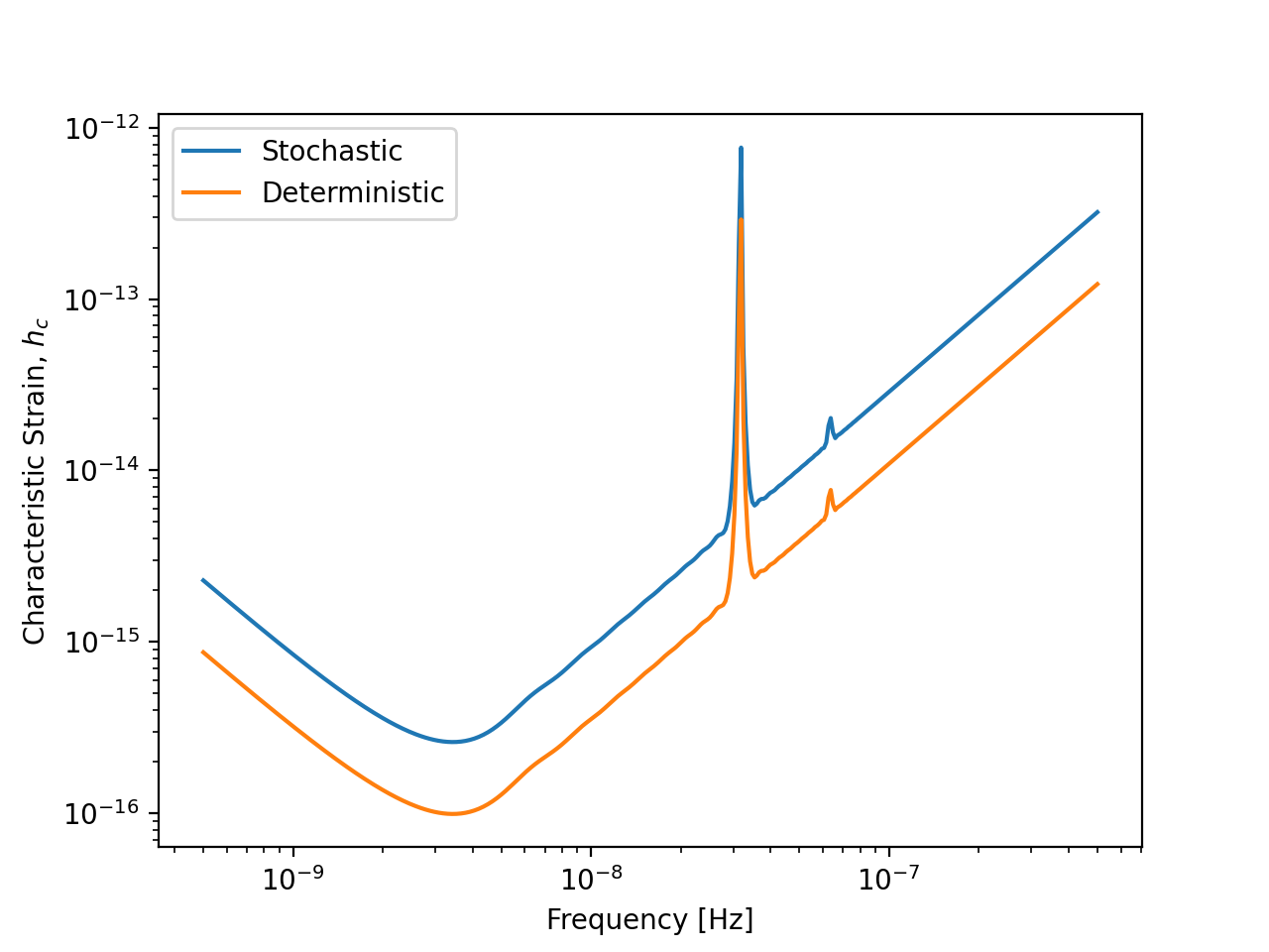
scGWB = sens.GWBSensitivityCurve(spectra)
scDeter = sens.DeterSensitivityCurve(spectra)
(Source code, png, hires.png, pdf)
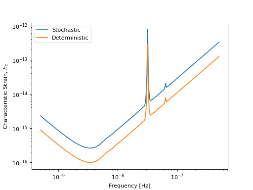
Comparison of a sensitivity curve for a deterministic and stochastic gravitational wave signal.
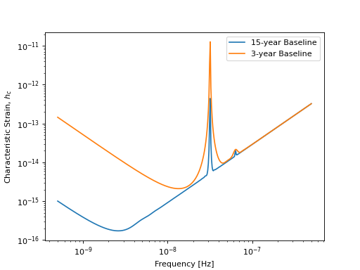
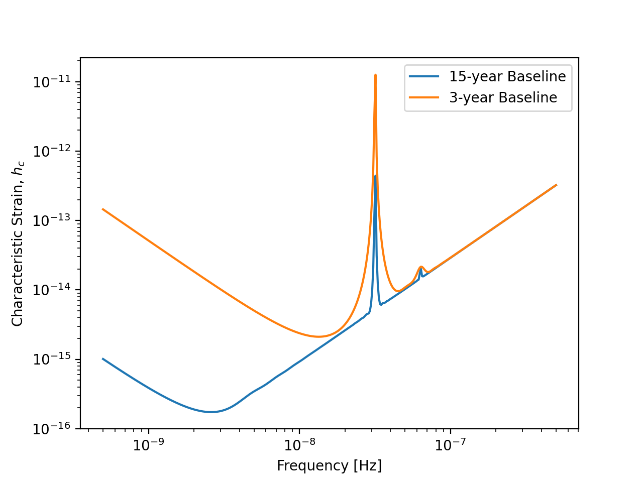
Compare this to a set of sensitivity curves made with 3-year pulsar baselines:
psrs2 = sim.sim_pta(timespan=3.0, cad=23, sigma=1e-7,
                    phi=phi, theta=theta, Npsrs=34)

spectra2 = [sens.Spectrum(p, freqs=freqs) for p in psrs2]
scGWB2 = sens.GWBSensitivityCurve(spectra2)
(Source code, png, hires.png, pdf)
