Note
This tutorial was generated from a Jupyter notebook that can be downloaded here.
SkySensitivity Tutorial
This tutorial is an introduction to the skymap module of the pulsar
timing array sensitivity curve package hasasia. For an introduction
to straight forward sensitivity curves see prior tutorials.
#Import the usual suspects.
import numpy as np
import matplotlib.pyplot as plt
%matplotlib inline
# You'll need these packages to make the skymaps and deal with units.
import healpy as hp
import astropy.units as u
import astropy.constants as c
#Import the needed modules.
import hasasia.sensitivity as hsen
import hasasia.sim as hsim
import hasasia.skymap as hsky
import matplotlib as mpl
mpl.rcParams['figure.dpi'] = 300
mpl.rcParams['figure.figsize'] = [5,3]
mpl.rcParams['text.usetex'] = True
#Make a set of random sky positions
phi = np.random.uniform(0, 2*np.pi,size=33)
cos_theta = np.random.uniform(-1,1,size=33)
theta = np.arccos(cos_theta)

#Adding one well-placed sky position for plots.
phi = np.append(np.array(np.deg2rad(60)),phi)
theta = np.append(np.array(np.deg2rad(50)),theta)

#Define the timsespans and TOA errors for the pulsars
timespans = np.random.uniform(3.0,11.4,size=34)
Tspan = timespans.max()*365.25*24*3600
sigma = 1e-7 # 100 ns
Here we use the sim_pta method in the hasasia.sim module to
simulate a set of hasasia.senstivity.Pulsar objects. This function
takes either single values or lists/array as inputs for the set of
pulsars.
#Simulate a set of identical pulsars, with different sky positions.
psrs = hsim.sim_pta(timespan=11.4, cad=23, sigma=sigma,
                    phi=phi, theta=theta)
Next define the frequency range over which to characterize the spectra
for the pulsars and enter each Pulsar object into a
hasasia.sensitivity.Spectrum object.
freqs = np.logspace(np.log10(1/(5*Tspan)),np.log10(2e-7),500)
spectra = []
for p in psrs:
    sp = hsen.Spectrum(p, freqs=freqs)
    sp.NcalInv
    spectra.append(sp)
Note above that we have called sp.NcalInv, which calculates the
inverse-noise-weighted transmission function for the pulsar along the
way. For realistic pulsars with +100k TOAs this step will take the most
time.
Define a SkySensitivity Object
Before defining a hasasia.skymap.SkySensitivity object we will need
to choose a set of sky locations. Here we use the healpy Python
package to give us a healpix pixelation of the sky.
#Use the healpy functions to get the sky coordinates
NSIDE = 32
NPIX = hp.nside2npix(NSIDE)
IPIX = np.arange(NPIX)
theta_gw, phi_gw = hp.pix2ang(nside=NSIDE,ipix=IPIX)
Next enter the list of Spectrum objects and the sky coordinates into
the SkySensitivity class.
SM=hsky.SkySensitivity(spectra,theta_gw, phi_gw)
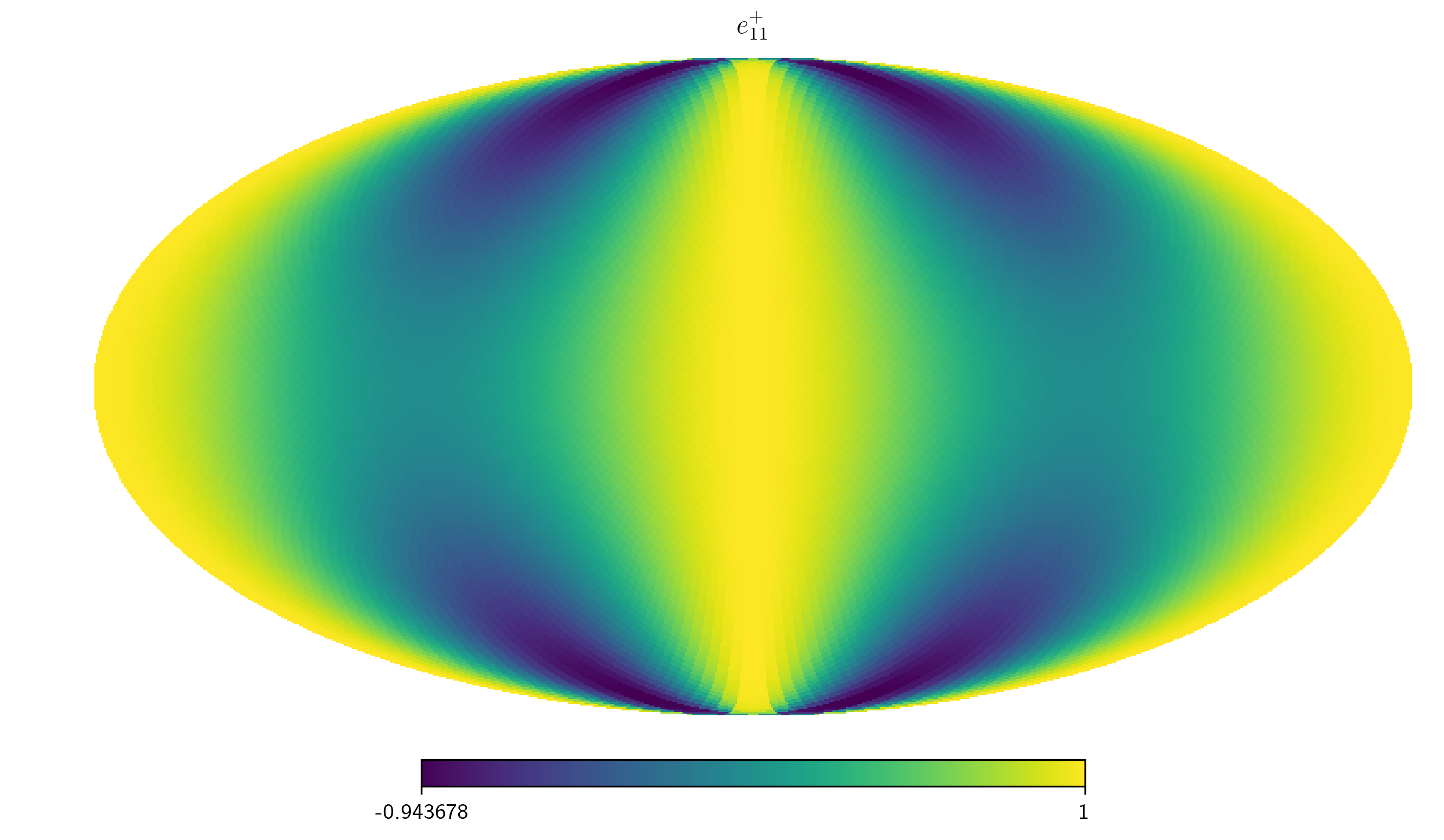
The SkySensitivity class has a number of accessible attributes and
methods. The polarization tensors :math:e^+ and :math:e^- are
available.
hp.mollview(SM.eplus[1,1,:], title='$e_{11}^+$',)
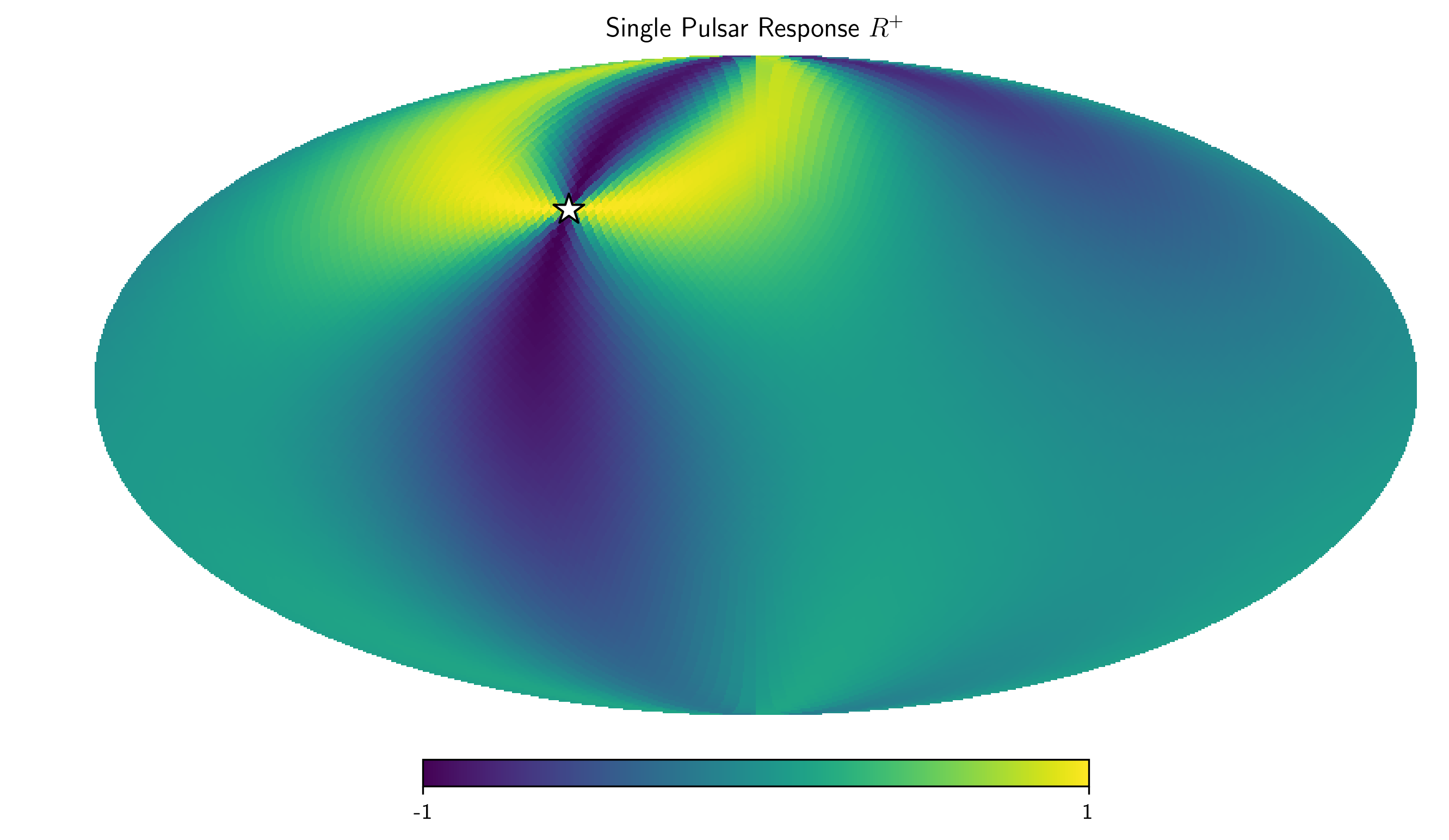
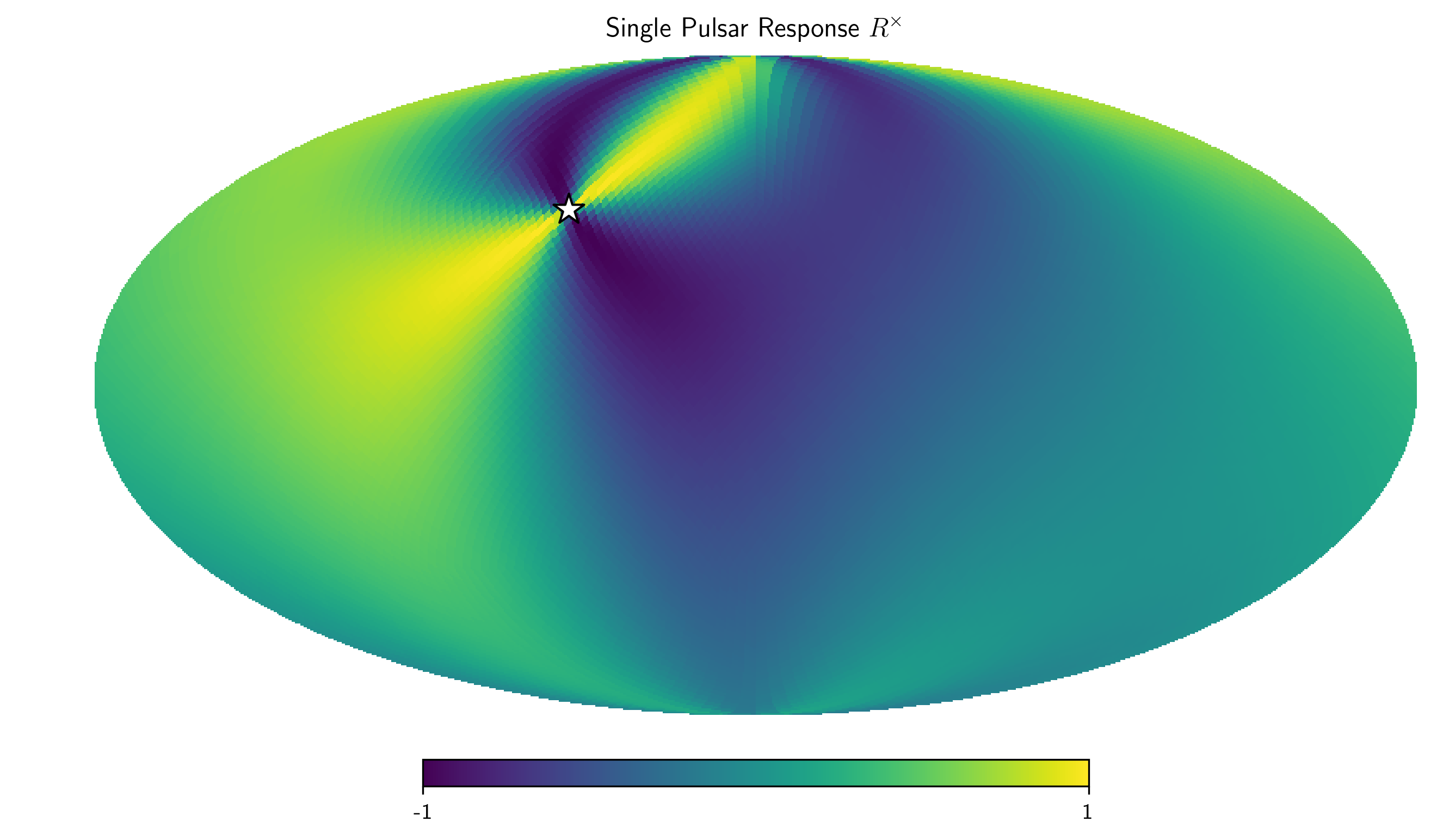
One can also access the residual response functions for each of the
individual pulsars, as SkySensitivity.Rplus and
SkySensitivity.Rcross.
idx = 0
hp.mollview(SM.Rplus[idx], fig=1,
            title="Single Pulsar Response $R^+$",min=-1,max=1)
hp.visufunc.projscatter(SM.thetas[idx],SM.phis[idx],
                        marker='*',color='white',
                        edgecolors='k',s=200)
hp.mollview(SM.Rcross[idx], fig=2,
            title=r"Single Pulsar Response $R^\times$",min=-1,max=1)
hp.visufunc.projscatter(SM.thetas[idx],SM.phis[idx],
                        marker='*',color='white',
                        edgecolors='k',s=200)

plt.show()
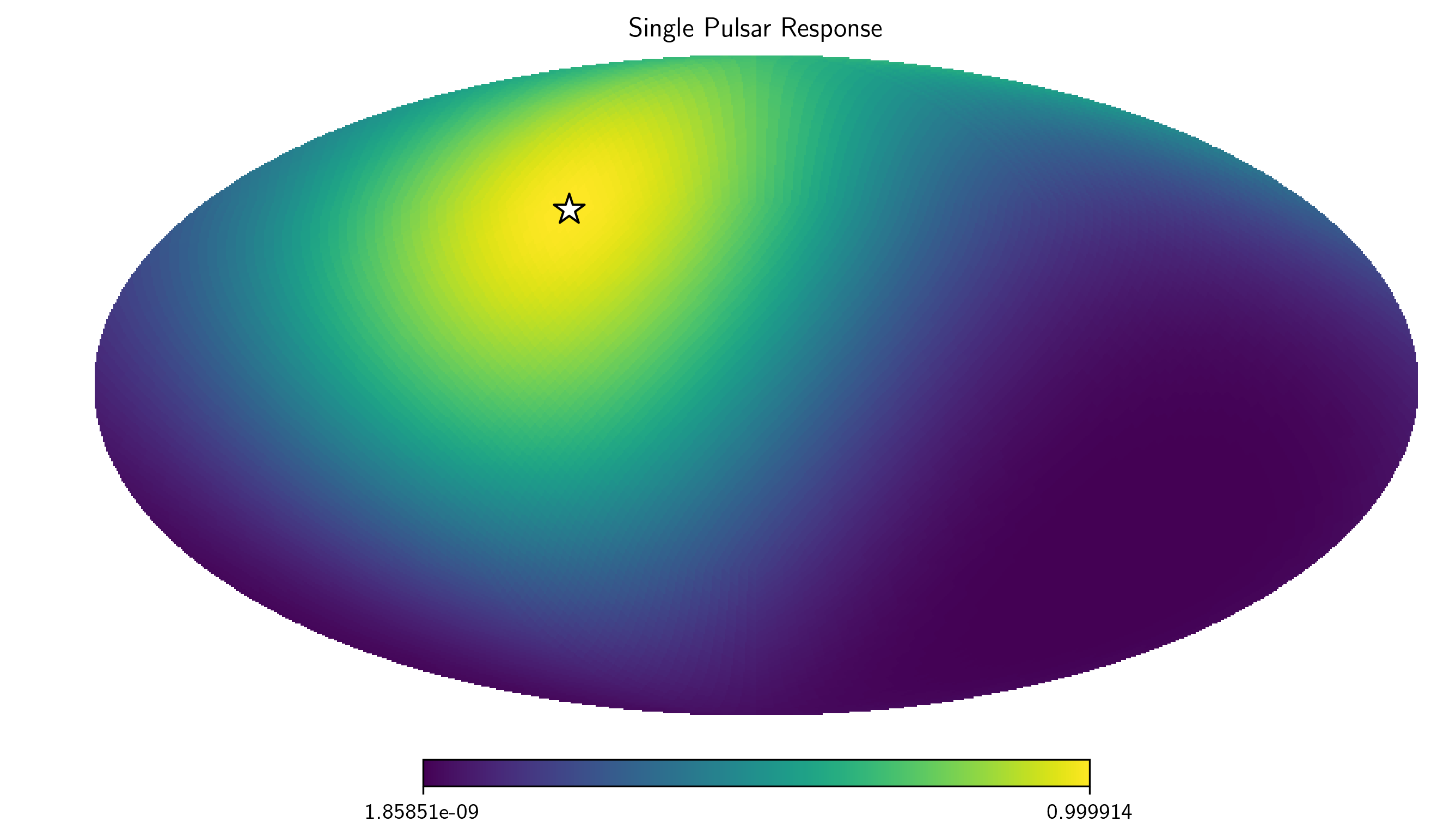
And the full residual response as SkySensitivity.sky_response.
idx =0
hp.mollview(SM.sky_response[idx], title="Single Pulsar Response")
hp.visufunc.projscatter(SM.thetas[idx], SM.phis[idx],
                        marker='*',color='white',
                        edgecolors='k',s=200)
plt.show()
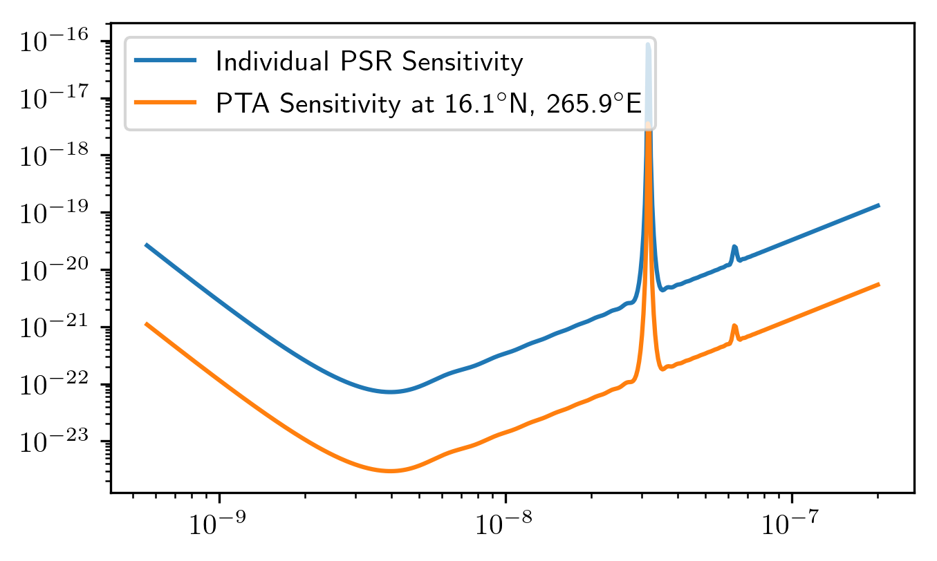
The full frequency and sky location sensitivity information is available
as SkySensitivity.S_effSky. The first index is across frequency,
while the second index is across sky position. Here we compare the
sensitivity from an individual pulsar to the full PTA’s senstivity at a
particular sky position.
sky_loc = 'PTA Sensitivity at '
sky_loc += '{0:2.1f}$^\circ$N, {1:2.1f}$^\circ$E'.format(np.rad2deg(theta_gw[252]),
                                               np.rad2deg(phi_gw[252]))
plt.loglog(SM.freqs,spectra[0].S_I, label='Individual PSR Sensitivity')
plt.loglog(SM.freqs,SM.S_effSky[:,252],
           label=sky_loc)
plt.legend(loc='upper left')
plt.show()
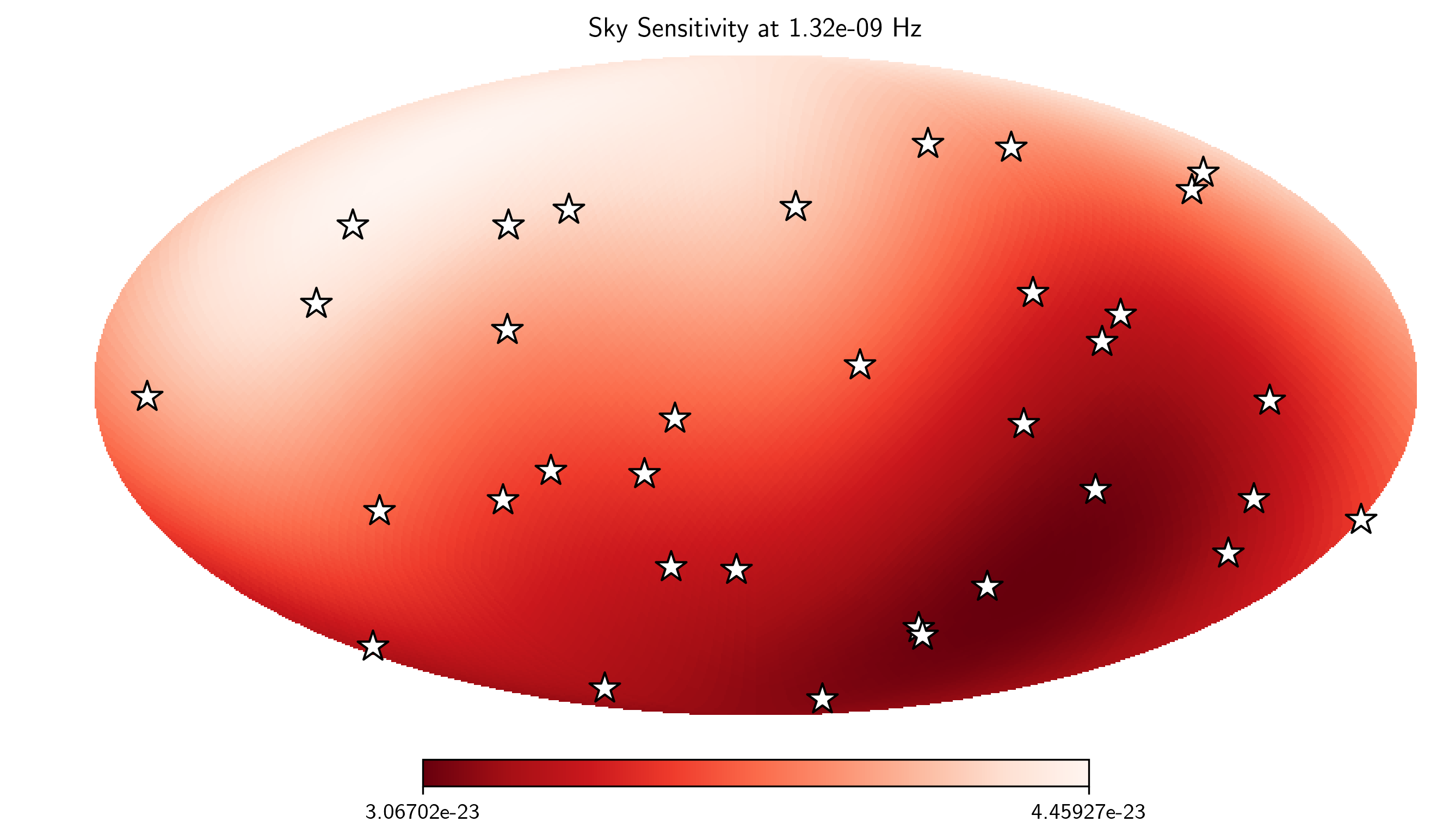
Here we plot the SkySensitivity.S_effSky across the sky at a given
frequency.
idx = 73
hp.mollview(SM.S_effSky[idx],
            title="Sky Sensitivity at {0:2.2e} Hz".format(SM.freqs[idx]),
            cmap='Reds_r')
hp.visufunc.projscatter(SM.thetas,SM.phis,
                        marker='*',color='white',
                        edgecolors='k',s=200)
plt.show()
Calculating SNR across the Sky
The SkySensitivity.S_effSky class comes with a method for
calculating the signal-to-noise ratio for a given signal. Rather than
calculate a signal from a single sky position, the method will calculate
the SNR from every sky position initially provided, given a particular
signal provided in strain across the frequency band.
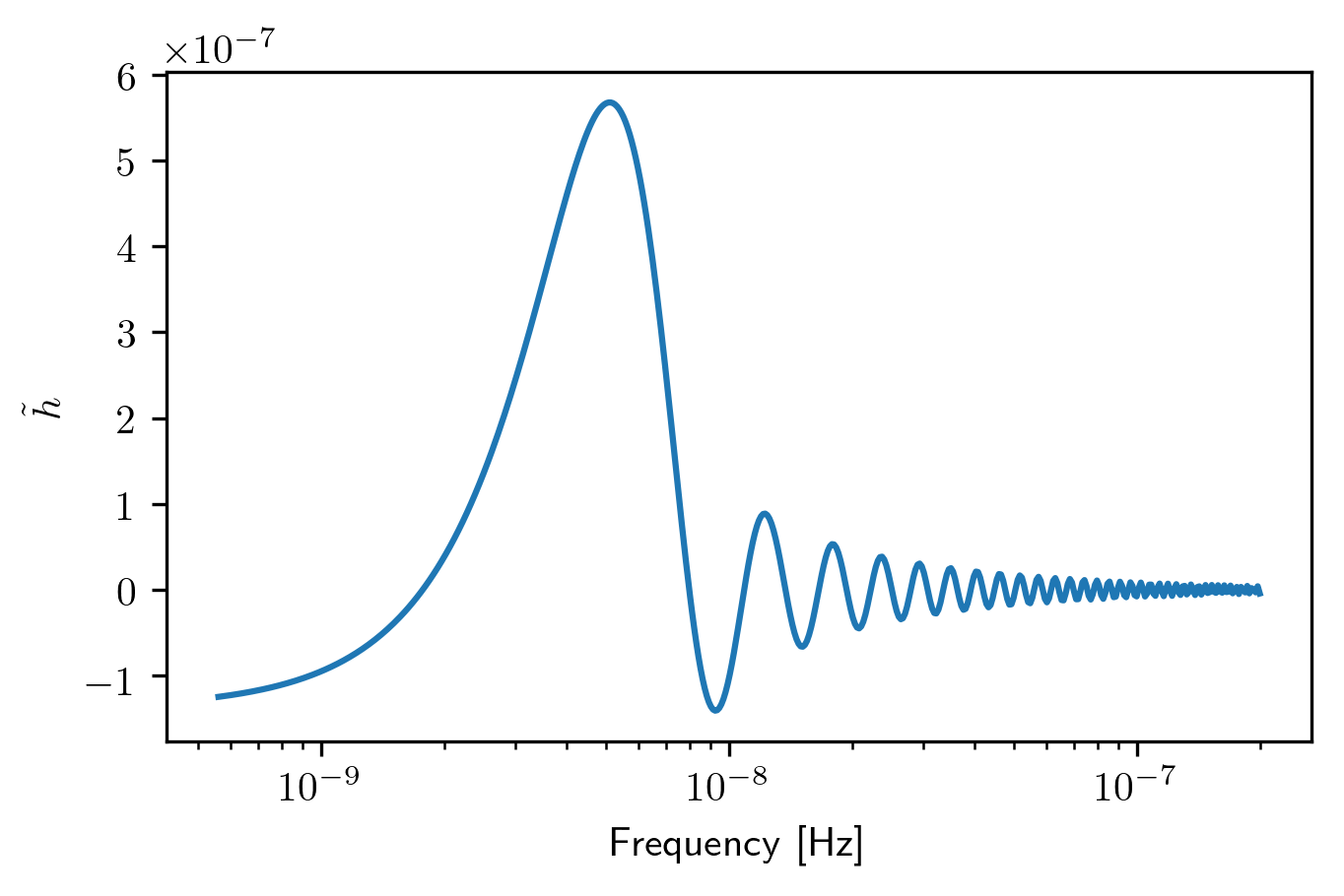
There is a convenience function for circular binaries provided as
hasasia.skymap.h_circ.
hCirc = hsky.h_circ(1e9,200,5e-9,Tspan,SM.freqs).to('')
Here we plot the signal in the frequency domain, for a finite integration time provided as the time span of the data set.
plt.semilogx(SM.freqs, hCirc)
plt.xlabel('Frequency [Hz]')
plt.ylabel(r'$\tilde{h}$')
plt.show()
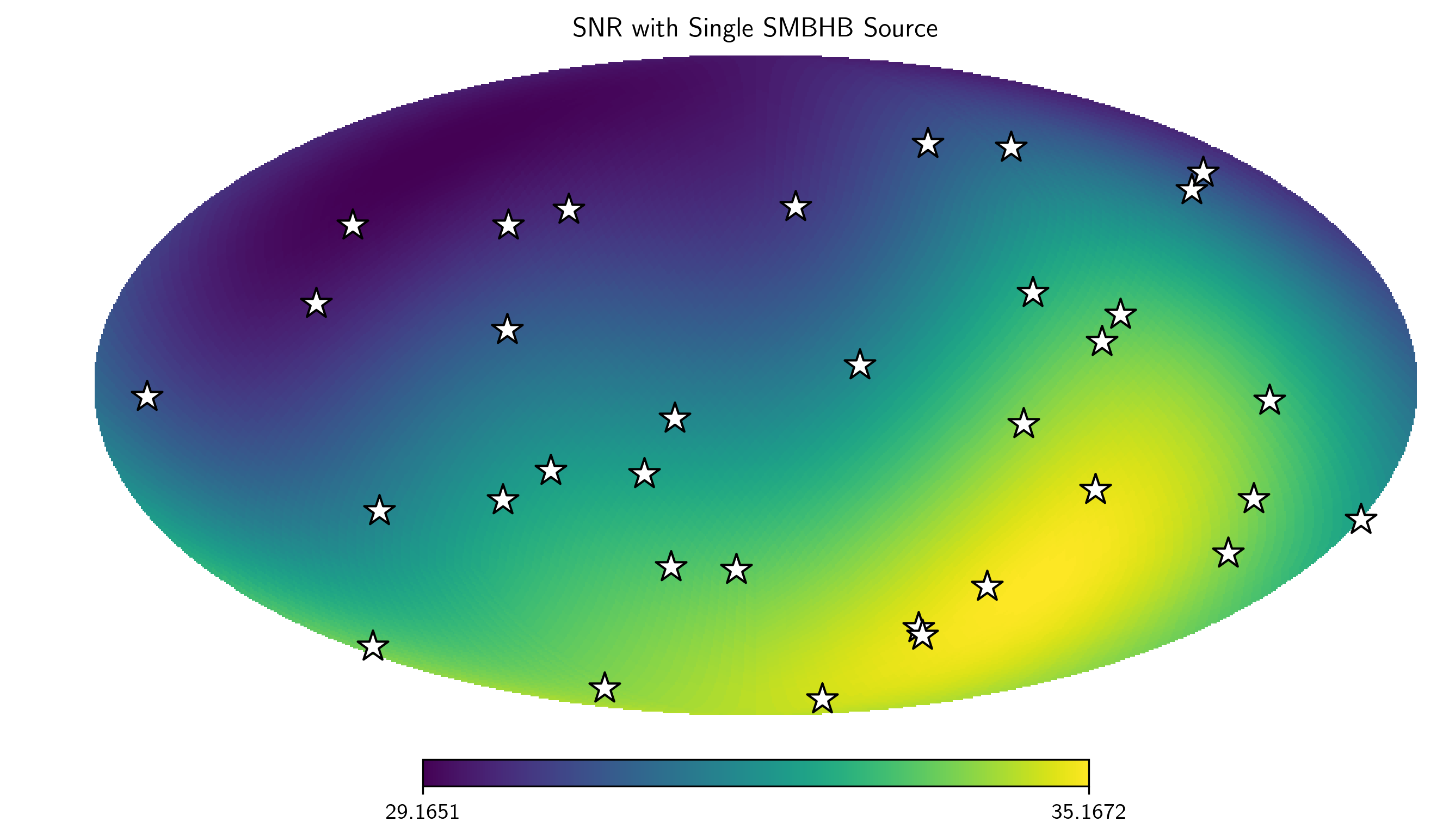
SNR = SM.SNR(hCirc.value)
idx = 167
hp.mollview(SNR,
            title="SNR with Single SMBHB Source",
            cmap='viridis')
hp.visufunc.projscatter(SM.thetas,SM.phis,marker='*',
                        color='white',edgecolors='k',s=200)
plt.show()
h_divA = (hsky.h_circ(1e9,200,5e-9,Tspan,SM.freqs)
          /hsky.h0_circ(1e9,200,5e-9)).value
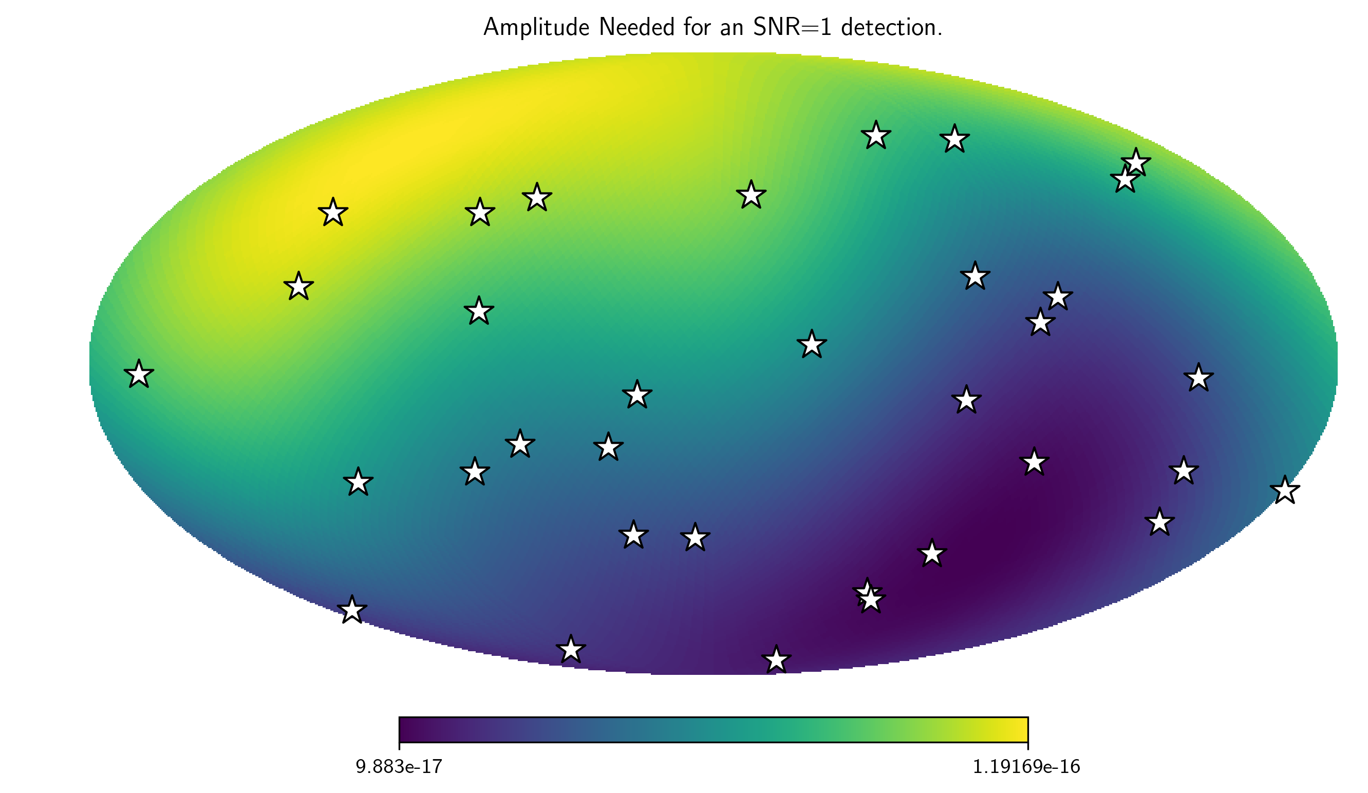
Amp = SM.A_gwb(h_divA)
hp.mollview(Amp,
            title="Amplitude Needed for an SNR=1 detection.",
            cmap='viridis')
hp.visufunc.projscatter(SM.thetas,SM.phis,marker='*',
                        color='white',edgecolors='k',s=200)
plt.show()